Earth’s Axial Tilt Vector Illustration Showing Earth’s Rotation, Seasons, and Sunlight Angle
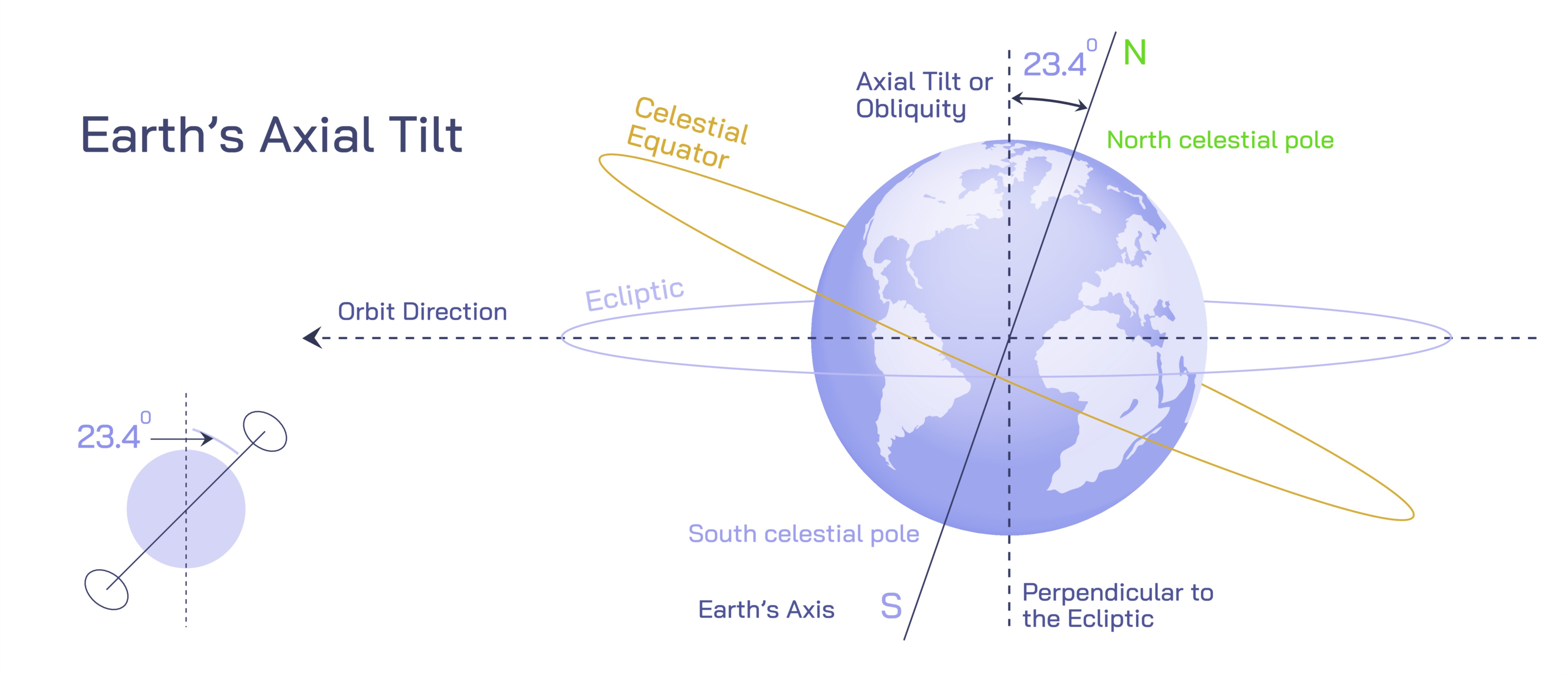
Earth’s axial tilt, also known as obliquity, is the angle between the planet’s rotational axis and its orbital plane around the Sun, approximately 23.5 degrees. This tilt is the primary reason for seasonal variations, changing day lengths, and fluctuations in solar intensity across the globe. A vector illustration of Earth’s axial tilt typically combines the depiction of the planet’s rotation, the orientation of its axis, the path of the Sun’s rays, and the resulting seasonal changes, providing a comprehensive understanding of how a simple tilt governs complex climatic patterns and environmental phenomena. By visualizing Earth’s tilt, rotation, and the movement around the Sun simultaneously, one can understand the cyclic nature of seasons and the variation in solar energy received at different latitudes over the course of a year.
At the core of such an illustration is the Earth’s axis, an imaginary line running from the North Pole to the South Pole. Unlike a vertical line perpendicular to the orbital plane, the axis is tilted 23.5 degrees relative to the perpendicular of Earth’s orbital plane, known as the ecliptic plane. In a vector diagram, the axis is usually represented as a straight line passing through the center of the globe, with arrows indicating the direction of rotation from west to east. This tilt remains nearly constant throughout the year due to the phenomenon of axial stability, allowing consistent seasonal patterns. The axis also defines the orientation of the planet in space, which in combination with Earth’s orbit around the Sun, determines which hemisphere receives more direct sunlight at any given time.
The rotation of the Earth on its tilted axis is another critical component in the illustration. The planet spins from west to east, completing a full rotation every 24 hours, producing the diurnal cycle of day and night. In vector illustrations, arrows or curved lines around the globe indicate this rotational direction, showing how different regions move in and out of sunlight. The tilt combined with rotation explains why the Sun appears higher in the sky during summer and lower during winter, and why daylight hours vary with latitude and season. By overlaying rotational motion on the tilted axis, the diagram allows viewers to understand the dynamic interplay between rotation and axial orientation.
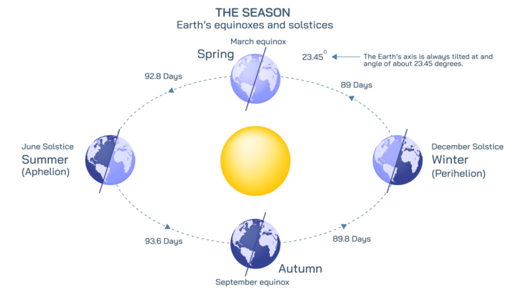
A central feature of the vector illustration is the Sunlight angle. Because of the axial tilt, the Sun’s rays strike the Northern and Southern Hemispheres at varying angles throughout the year. During the June solstice, the North Pole tilts toward the Sun, resulting in direct sunlight over the Tropic of Cancer and longer daylight hours in the Northern Hemisphere. Conversely, during the December solstice, the South Pole tilts toward the Sun, with maximum solar intensity over the Tropic of Capricorn, giving the Southern Hemisphere its summer and the Northern Hemisphere its winter. In vector diagrams, sunlight is represented as parallel rays striking the tilted Earth, often with arrows indicating the direction of solar radiation and shading to highlight intensity variations. This visual clearly demonstrates why the equator experiences relatively consistent sunlight year-round, whereas polar regions undergo extreme seasonal variation.
Seasons are an immediate consequence of Earth’s axial tilt and orbit around the Sun. In vector illustrations, the Earth is often shown at four positions along its elliptical orbit to depict spring equinox, summer solstice, autumn equinox, and winter solstice. At equinoxes, the tilt is oriented perpendicular to the Sun-Earth line, resulting in nearly equal day and night lengths across all latitudes. At solstices, one hemisphere receives maximum sunlight while the other is in prolonged darkness. By marking the equator, Tropic of Cancer, Tropic of Capricorn, Arctic Circle, and Antarctic Circle, vector diagrams connect axial tilt with the latitudinal distribution of solar energy, illustrating phenomena such as the Midnight Sun and polar night.
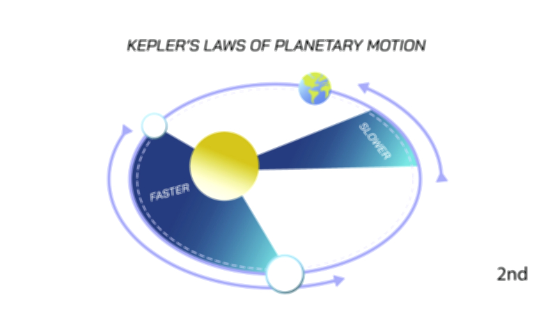
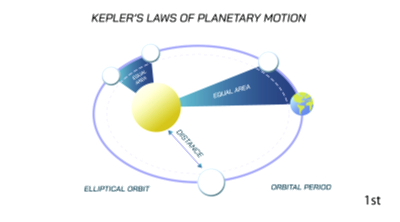
The illustration may also depict Earth’s orbital path, emphasizing that the tilt remains fixed relative to distant stars rather than the Sun, producing a consistent seasonal cycle as Earth moves around the Sun. The orbital depiction can include the Sun at the center, with Earth’s position labeled for each solstice and equinox, showing how axial orientation influences the hemispheric exposure to sunlight. This clarifies why the distance from the Sun is not the main driver of seasons; instead, it is the angle of solar incidence due to axial tilt.
Vector diagrams often incorporate daylight variation patterns, showing how the length of the day increases or decreases with latitude and season. Arcs or shading may illustrate the Sun’s apparent path in the sky for different times of the year. Similarly, arrows may indicate the intensity of solar radiation received at various points, highlighting why the tropics remain warm while polar regions experience extreme cold and variation. Such diagrams link the geometric tilt to observable climatic patterns, helping viewers understand why axial tilt is critical for life on Earth, agriculture cycles, and climate zones.
Advanced illustrations may also include axial precession, the slow wobble of Earth’s rotation axis over approximately 26,000 years, or nutation, a shorter-term oscillation in tilt. While subtle, these phenomena influence long-term climate patterns, such as glacial and interglacial periods. Vector diagrams can show precession with a circular arrow around the axis to represent the gradual movement, providing context for Earth’s axial dynamics beyond seasonal cycles.
Overall, a vector illustration of Earth’s axial tilt combines multiple layers of information: the 23.5-degree tilt, rotational direction, Sun-Earth geometry, seasonal positions along the orbit, sunlight angles, and latitudinal daylight variation. By integrating these elements, the diagram allows viewers to visualize how axial tilt governs the cycle of seasons, the variation in solar energy distribution, and the observable changes in day length and sunlight angle across the globe. Such illustrations are crucial in geoscience, astronomy, and education, providing a clear and comprehensive understanding of the fundamental mechanics that regulate Earth’s climate system, seasonal rhythms, and the distribution of life-sustaining solar energy.
This type of vector illustration also emphasizes the broader implications of axial tilt: it explains how consistent seasons arise, how the tilt affects climatic zones, and why the tropics remain relatively stable while higher latitudes experience significant seasonal variation. It connects geometric principles to tangible environmental outcomes, showing the intersection of planetary motion, solar energy, and life on Earth. By highlighting rotation, tilt, and sunlight geometry, the illustration bridges abstract astronomical concepts with observable terrestrial phenomena, making the physics of Earth’s motion intuitive and visually accessible.
The combination of axis depiction, orbital positions, solar angles, and seasonal variations provides an educational tool that communicates not only the geometric orientation of the planet but also the dynamic processes that arise from that orientation. From understanding agriculture patterns and climate systems to explaining daylight variation and solar intensity, the vector illustration of Earth’s axial tilt serves as a complete visual framework for appreciating how a single physical characteristic—the 23.5-degree tilt—regulates so many aspects of life and environmental behavior on the planet.