𝐒𝐢𝐱 𝐏𝐫𝐨𝐛𝐚𝐛𝐢𝐥𝐢𝐭𝐲 𝐃𝐢𝐬𝐭𝐫𝐢𝐛𝐮𝐭𝐢𝐨𝐧𝐬 𝐮𝐬𝐞𝐝 𝐢𝐧 𝐒𝐭𝐚𝐭𝐢𝐬𝐭𝐢𝐜𝐬 — 𝐃𝐞𝐞𝐩 𝐄𝐝𝐮𝐜𝐚𝐭𝐢𝐨𝐧𝐚𝐥 𝐂𝐨𝐧𝐜𝐞𝐩𝐭 𝐒𝐮𝐦𝐦𝐚𝐫𝐲.
Probability distributions are among the most important conceptual tools in statistics because they describe how random variables behave under uncertainty. They serve as structured maps that convert randomness into patterns, making it possible to predict, analyze, and interpret outcomes in scientific experiments, business forecasting, manufacturing quality control, medicine, psychology, economics, machine learning, and countless other fields. While many probability distributions exist, six of them are used with particular frequency in statistical analysis because they each represent a category of real-world random behaviour. These distributions include the Normal distribution, Binomial distribution, Poisson distribution, Exponential distribution, Uniform distribution, and Student’s t-distribution. Each one captures a specific type of uncertainty—some model continuous variables that cluster around an average, others describe binary outcomes, arrival counts, waiting times, or sample-based uncertainty. Learning these six distributions does not simply add six formulas to memory; instead, it builds the foundation for understanding how randomness manifests in different environments and how statistics transform data into knowledge.
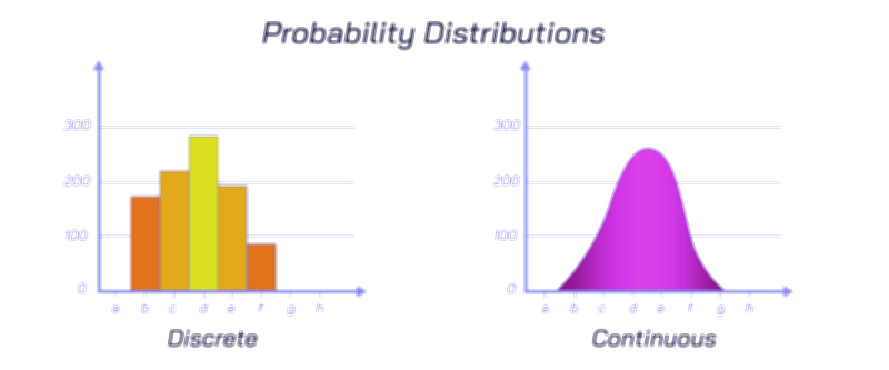
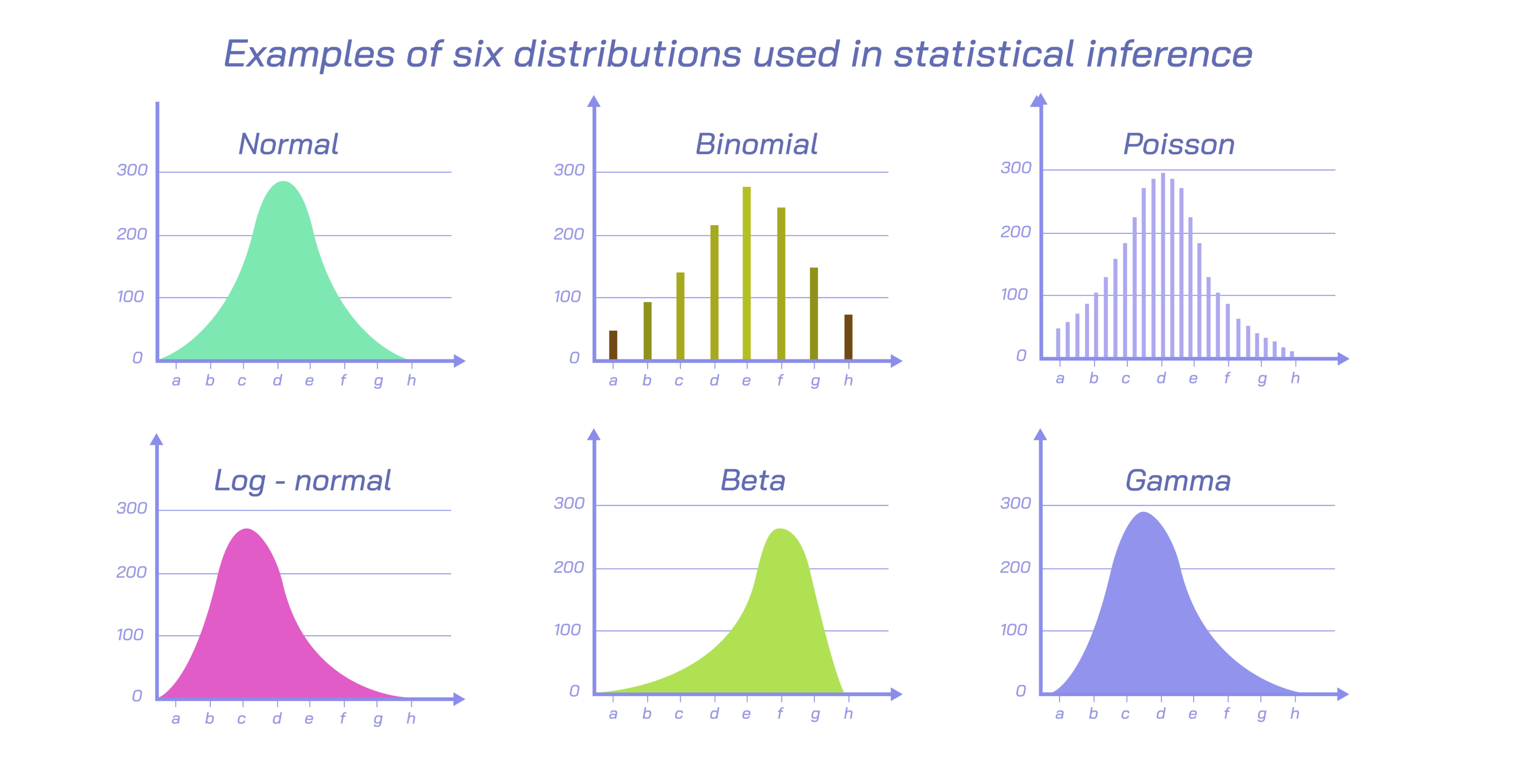
Among the six types, the Normal distribution—often recognized by its smooth bell-shaped curve—is the most widely observed in natural and social systems. It arises when many small, independent influences accumulate to produce a final outcome, causing most results to cluster near the mean with fewer observations falling far above or below it. The normal distribution describes phenomena such as heights, IQ scores, weights of newborns, exam performance, biological traits, blood pressure levels, and measurement errors in scientific experiments. Its symmetry makes it powerful for interpreting averages and variations, and it serves as the backbone of inferential statistics because many statistical tests assume that sampled data follows or approximates a normal distribution. The central limit theorem further emphasises the importance of the normal distribution by demonstrating that when independent random variables are added, their combined distribution tends to approach normality—even if the original variables were not normally distributed. Because of this deep connection with reality and statistical theory, the normal distribution becomes the benchmark for comparing patterns of variation in fields ranging from engineering to finance to psychology.
A second crucial distribution among the six is the Binomial distribution, which applies when an event has only two possible outcomes—commonly described as success or failure—and the event is repeated a fixed number of times. The binomial distribution therefore models the probability of achieving a specific number of successes across repeated independent attempts. This pattern appears widely in clinical trials, quality testing, educational assessment, genetics, and polling. For example, the binomial distribution describes how many patients recover after treatment, how many manufactured items pass inspection out of a batch, how many correct answers a student gets on a true-or-false exam, or how many families support a candidate during an election survey. The core of the binomial distribution lies in two pieces of information: the number of trials and the probability of success for each trial. These two elements work together to provide a detailed understanding of how likely each possible outcome is, guiding decision-making in fields that depend on estimating success rates or proportions accurately.
Closely related yet fundamentally different in function is the Poisson distribution, which models the number of random events occurring in a fixed period of time or space rather than in a fixed number of trials. With the Poisson distribution, the question becomes “how many events will occur during the next hour?” rather than “how many successes will occur in ten attempts?” The Poisson distribution models situations such as the number of cars arriving at a toll gate every minute, the number of calls received by a customer service centre per hour, the number of defects per page in printed material, or the number of earthquakes exceeding a certain magnitude per year. The key requirement for the Poisson distribution is that events occur independently and at a steady average rate. When these criteria are satisfied, the Poisson distribution becomes a reliable tool for forecasting workloads, planning emergency resources, estimating accident probabilities, designing transportation systems, and calculating insurance risks. Because many everyday processes consist of random arrivals or occurrences over time, the Poisson distribution is deeply woven into operations research and risk analysis.
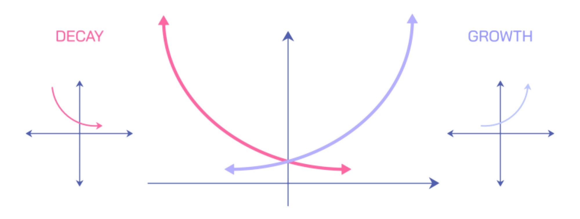
The Exponential distribution expands naturally from the Poisson distribution and represents one of the most meaningful interpretations of randomness in time. Whereas the Poisson distribution counts how many events occur per interval, the exponential distribution describes the expected waiting time between consecutive events when they occur continuously and independently at a constant average rate. This distribution emerges in scenarios such as the time until a machine fails, the time until the next power outage, the lifespan of electronic components, the waiting time for a bus at a station, and even the decay of radioactive particles. One remarkable property of the exponential distribution is that it is “memoryless,” meaning that the probability of an event occurring soon does not depend on how much time has already passed. For example, if a bulb has not yet burned out after five months, the probability that it will fail in the next week remains the same as it was from the very beginning. This makes the exponential distribution an indispensable tool in reliability engineering, survival analysis, risk management, and optimization of service systems.
Another major distribution used widely in statistical modelling is the Uniform distribution, which describes situations where every outcome within a certain range is equally likely. Unlike the normal distribution—with its central clustering—or the exponential distribution—with its time-dependent decay, the uniform distribution spreads probability evenly. It represents ideal randomness when no outcome has an inherent advantage or bias. Examples include selecting a random number from a range, predicting where a dart thrown at a board might land, or simulating equally likely environmental states in computer models. The uniform distribution is especially significant in computational sciences because random sampling in simulations, encryption, Monte-Carlo experiments, and artificial intelligence often begins by generating values drawn from a uniform distribution. It also illustrates a fundamental lesson about randomness: sometimes uncertainty is not weighted toward an average, but equally distributed across all possibilities.
The final distribution in this educational group of six is the Student’s t-distribution, which plays a central role in real-world data analysis, especially when sample sizes are small. While the normal distribution assumes that the sample closely represents the population, the t-distribution accounts for added uncertainty when the sample size is limited. It has heavier tails than the normal distribution, meaning it allows for a higher chance of extreme outcomes. This property makes the t-distribution more cautious and realistic when working with small datasets, which are common in medicine, behavioural science, field research, prototype testing, and early-stage product experiments. The t-distribution forms the basis of the t-test, one of the most widely used statistical procedures for determining whether observed differences between groups are meaningful or due to chance. Whenever sample sizes are small or population variability is unknown, the t-distribution replaces the normal distribution to protect the reliability of statistical conclusions.
Studying these six distributions reveals an essential truth about probability theory: uncertainty behaves in predictable patterns rather than random chaos. Each of the six major distributions represents a different kind of uncertainty—clustering around an average, counting successes, counting arrivals, waiting times, equal likelihood across ranges, and small-sample variability. Although the fields that use them may vary—from economics to biology, from psychology to engineering, from marketing to artificial intelligence—the mathematical forces underpinning randomness remain remarkably consistent. Knowing which distribution applies to a dataset allows statisticians and scientists to make informed inferences, forecast trends, quantify risks, evaluate hypotheses, and design better systems.
Together, these six probability distributions create a unified framework that transforms randomness into logical structure. They allow analysts to interpret what has happened, anticipate what may happen, and understand the forces driving variability. Whether evaluating medical treatments, optimizing supply chains, forecasting financial markets, improving product quality, studying human behaviour, or building predictive algorithms, these six distributions act as the foundation on which statistical thinking and data-driven decision-making are built.