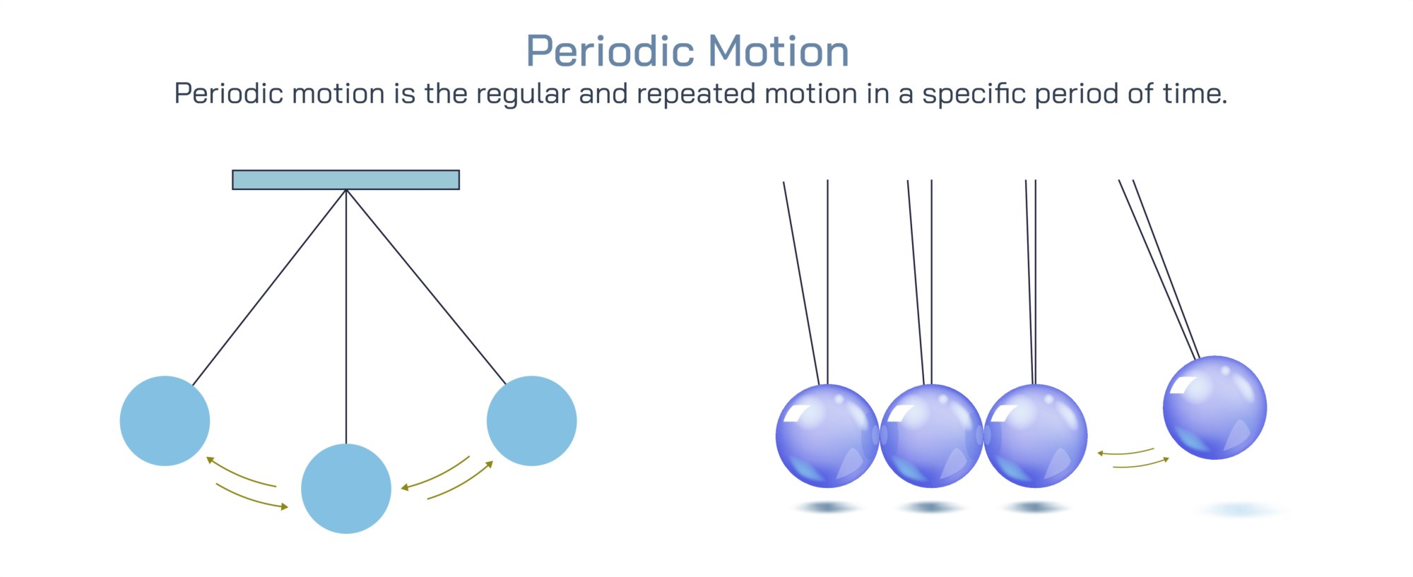
Periodic Motion Explained: Understanding Repetitive Movements in Physics with Examples
Periodic motion is a fundamental concept in physics that describes any motion that repeats itself at regular intervals of time. It is a cornerstone in understanding mechanical vibrations, waves, oscillations, and many natural and engineered systems. Objects in periodic motion exhibit cyclical behavior, returning to the same position, velocity, and acceleration after a fixed period. Common examples include pendulums, springs, planets orbiting stars, and vibrating strings. A vector illustration explaining periodic motion typically integrates motion paths, time intervals, displacement graphs, and examples of oscillatory systems, providing a clear and visually engaging representation. By combining labeled components, directional arrows, amplitude markers, and frequency indicators, such illustrations allow learners to grasp the nature, parameters, and applications of periodic motion.
At the center of the illustration is a generic oscillatory system, such as a mass-spring setup or a swinging pendulum. Labels identify key components: mass (m), spring (k), equilibrium position, amplitude (A), and restoring force (F) for the mass-spring system, or bob, string, pivot, amplitude (θ), and equilibrium position for the pendulum. Arrows along the motion path indicate the direction of movement, emphasizing the repetitive back-and-forth nature of the motion. Color-coded paths may represent different phases of oscillation, such as forward and backward swings, highlighting symmetry in periodic behavior.
The time period (T), the duration for one complete cycle of motion, is illustrated using circular arrows or wave graphs. Labels explain that T depends on system characteristics, such as mass and spring constant for a spring system (T = 2π√(m/k)) or length and gravity for a pendulum (T = 2π√(L/g)). Arrows connect physical parameters to time period, showing how changes in mass, spring stiffness, pendulum length, or gravitational acceleration affect oscillation frequency. Magnified insets may highlight one full cycle of motion, illustrating the start and end points, amplitude extremes, and equilibrium crossing.
Amplitude (A) and displacement (x) are visually represented along the oscillation path or on a sinusoidal displacement-time graph. Labels indicate maximum displacement from equilibrium (amplitude), instantaneous displacement, and oscillation direction. Color gradients along the path may represent the magnitude of displacement, providing a clear visual cue for the extent of motion. Arrows indicate velocity and acceleration directions at different points, emphasizing that maximum speed occurs at equilibrium while maximum acceleration occurs at extreme positions.
Vector illustrations often include velocity and acceleration diagrams, showing that in periodic motion, velocity and acceleration are sinusoidally varying and phase-shifted relative to displacement. Arrows along the graphs indicate the direction of velocity and acceleration vectors, with labels highlighting key points: zero velocity at maximum displacement and maximum acceleration pointing toward the equilibrium position. Magnified insets may illustrate the relationship between force and acceleration vectors in restoring motion, reinforcing Newton’s second law in oscillatory systems.
Additional examples are incorporated for educational clarity. Pendulums, mass-spring systems, tuning forks, planetary orbits, and vibrating guitar strings are depicted, each labeled with motion type, amplitude, period, and frequency. Arrows indicate repetitive motion and cycles, while color-coded overlays distinguish between different systems. Insets may show real-world applications, such as clocks using pendulums, seismic oscillations, and musical instruments, linking abstract concepts to practical contexts.
The illustration may also include frequency (f = 1/T) and angular frequency (ω = 2πf) indicators, showing the inverse relationship between time period and frequency. Arrows and labels indicate how higher frequency corresponds to shorter time periods, providing a connection between oscillation speed and practical systems like electrical signals, sound waves, and mechanical vibrations.
Vector diagrams often incorporate energy transformations in periodic motion. Arrows and labels illustrate kinetic energy and potential energy exchange, showing maximum kinetic energy at equilibrium and maximum potential energy at extreme positions. Color gradients along the motion path visually indicate energy conversion, helping learners understand the conservation of mechanical energy in ideal oscillatory systems.
By combining oscillatory paths, time period and frequency indicators, displacement, velocity, acceleration graphs, amplitude markers, and real-world examples, a vector illustration of periodic motion provides a comprehensive, visually intuitive understanding. Color coding, labeled arrows, and magnified insets make abstract oscillatory behavior clear and easy to relate to both theory and application.
Ultimately, a periodic motion vector illustration demonstrates the repetitive nature of physical motion, the interrelationship of displacement, velocity, acceleration, and energy, and the influence of system parameters on oscillation. Through labeled components, directional arrows, sinusoidal graphs, and examples from daily life and physics experiments, the diagram transforms a fundamental physical concept into an educational, visually engaging, and intuitive learning tool for students, educators, and science enthusiasts.